论文阅读：Control Theoretic Approach to Fine-Tuning and Transfer Learning

24th Sep 2025
14 min read
Tags:
Fine Tuning,
Catastrophic Forgetting

Original Paper: [2404.11013] Control Theoretic Approach to Fine-Tuning and Transfer Learning

Preliminaries

Hausdorff Space: A topological space $(X, \mathcal{T})$ is said to be a Hausdorff space if

$$ \forall x,y\in X,x\neq y\Longrightarrow\exists U,V\in\mathcal{T}\mathrm{~s.t.~}x\in U,y\in V,\mathrm{~and~}U\cap V=\emptyset $$

where $\mathcal{T}$ is the set of all the open sets in the space.

Hausdorff 空间保证了点的可分离性。

Basis of Topological Spaces: The basis of a topological space $\mathcal{B}$ is a set of open sets satisfying

$$ \exists\mathcal{B}=\{B_1,B_2,B_3,\ldots\}\subseteq\mathcal{T}\mathrm{~s.t.~}\forall U\in\mathcal{T},U=\bigcup_{i\in I}B_i\text{ for some }I $$

Second-Countable: A topological space $(X, \mathcal{T})$ is said to be second countable if $\mathcal{T}$ has a countable basis.

Homeomorphism: A mapping $\phi: U \to V$ is homeomorphism if both $\phi$ and $\phi^{-1}$ are continuous mapping.

Locally Euclidean and Chart: A topological space $X$ is said to be locally Euclidean if for any $p \in X$, there exists an open neighbor $U$ of $p$, a open set $V \subseteq \mathbb{R}^n$, and a homeomorphism $\phi$ such that

$$ \phi: U \to V. $$

Here $\phi$ is called the chart.

流形上每个局部都可以被坐标卡 chart 映射到一块 $\mathbb{R}^n$ 的区域

Topological Manifold: An $n$-dimensional topological manifold is a topological space that is Hausdorff, second-countable, and locally Euclidean of dimension $n$.

Smooth Curve: A smooth curve at a point $p$ on an manifold $M$ is a smooth map $\gamma: I \to M$, where $I \subseteq \mathbb{R}$ is an open interval containing $0$, such that $\gamma(0) = p$.

Equivalence Relation on Curves: Let $(U, \phi)$ be a local chart containing the point $p$, where $\phi: U \to \mathbb{R}^n$. Two smooth curves $\gamma_1$ and $\gamma_2$ at $p$ are said to be equivalent iff their velocity vectors in the chart coordinates are identical, that is

$$ \frac{\mathrm{d}}{\mathrm{d}t}(\phi\circ\gamma_1)(t)\bigg|_{t=0}=\frac{\mathrm{d}}{\mathrm{d}t}(\phi\circ\gamma_2)(t)\bigg|_{t=0}. $$

可以理解为切平面上一个方向的曲线是等价的

Tangent Vector: A tangent vector $v$ at a point $p$ is an equivalence class of all smooth curves passing through $p$. We denote this as $v = [\gamma]$.

Tangent Space: The tangent space at a point $p$ on $M$, denoted by $T_pM$, is the set of all tangent vectors at $p$:

$$ T_pM:=\{[\gamma]\mid\gamma:I\to M\text{ is a smooth curve with }\gamma(0)=p\} $$

Problem Statement

Dataset and System: Consider the paired sets $(\mathcal{X},\mathcal{Y})=\{(x^{i},y^{i})\}_{i=1}^{q}$ in a connected Riemannian manifold $\mathcal{M}$, where elements of $\mathcal{X}$ are pairwise distinct. We take the system

$$ \dot{x}(t)=f(u(t), x(t)), \quad u\in L_\infty([0,T],\mathbb{R}^{\bar{n}\times\bar{n}}) $$

$$ x^i\in\mathbb{R}^n \overset{E}{\operatorname*{\longrightarrow}} \bar{x}^i\in\mathbb{R}^{\bar{n}} \overset{\varphi_T(u,\cdot)}{\operatorname*{\longrightarrow}} \bar{y}^i\in\mathbb{R}^{\bar{n}} \overset{R}{\operatorname*{\longrightarrow}} y^i\in\mathbb{R}^{n_o} $$

where $E: \mathbb{R}^n \to \mathbb{R}^{\bar{n}}$ is an embedding function, $R: \mathbb{R}^{\bar{n}} \to \mathbb{R}^n$ is a readout function, $\bar{n}$ is the embedding dimension, $n_o$ is the output dimension, and $\varphi_t(u,\cdot)$ is the map generated by the control function $u$. For simplicity, we assume that $n = \bar{n}$, and let $R$ be the orthogonal projection, that is

$$ R:x\in\mathbb{R}^n\mapsto Cx\in\mathbb{R}^{n_o}, \quad \text{where} \quad C=[O_{n_{o}\times n-n_{o}}I_{n_{o}\times n_{o}}]\in\mathbb{R}^{n_{o}\times n}. $$

If $n = n_o$ and $R$ is the identity map, then we call the problem the control with fixed end-points（固定终值条件）. Otherwise, control with partially constrained end-points（终值约束条件）.

Objective (Memorization Property) : The control $u$ is said to have memorized the ensemble $(\mathcal{X}, \mathcal{Y})$ if the following holds for a finite $T \geq 0$:

$$ R(\varphi_T(u,E(x^i)))=y^i, \quad \forall x^i\in\mathcal{X}. $$

我们的总目标就是找到一个控制信号 $u$，对任意数据都能满足 memorization property。

Cost Functional: We define per-sample cost functional for a given point $x^i$ as

$$ \mathcal{J}^i(u)=\frac{1}{2}\|C\varphi(u,x^i)-y^i\|^2. $$

Then, the cost-functional for the entire ensemble is

$$ \mathcal{J}(u,\mathcal{X}):=\sum_{i=1}^{q}\|C\varphi(u,x^{i})-y^{i}\|^{2}+\lambda\int_{0}^{T}\|u(\tau)\|^{2}d\tau. $$

where $\lambda$ is some regularization coefficient.

q-Folded Method: Suppose $\mathcal{X}$ contains $q$ data points. Stack all the points in $\mathcal{X}$ into a vector of dimension $nq$ denoted by $X_0$, and the stacked outputs by $Y$. The minimization problem is

$$ \mathcal{J}(u,X_0):=\|\Lambda(C)\vec{\varphi}_T(u,X_0)-Y\|^2+\int_0^T\|u(\tau)\|^2d\tau. $$

$$ \text{subject to} \quad \dot{X}(t)=F(u(t),X(t)), \quad X(0)=X_0. $$

where $\Lambda(C):=\mathrm{diag}(C,\cdots,C)\in\mathbb{R}^{n_{0}q\times nq}$, and $F$ is the dynamics created by copying $f$ $q$-times.

使用 q-folded method 求解非常困难。

Existence of a Control Function

Lie Bracket: Let $g_1$ and $g_2$ be differentiable vector fields in $\mathcal{M} \subset \mathbb{R}^n$, we call the Lie bracket of $g_1$ and $g_2$ the vector field:

$$ g_1,g_2:=\frac{\partial g_2(x)}{\partial x}g_1(x)-\frac{\partial g_1(x)}{\partial x}g_2(x), \quad \mathrm{for} \quad x\in\mathcal{M} $$

Lie bracket 的核心含义：测量路径的不闭合程度，沿着以下两种路径：(1) 先 $g_1$ 走 $\epsilon$，再 $g_2$ 走 $\epsilon$；(2) $g_2$ 走 $\epsilon$，再 $g_1$ 走 $\epsilon$。两种路线到达的终点距离为：
$$ \epsilon^2\left(\frac{\partial g_2(x)}{\partial x}g_1(x)-\frac{\partial g_1(x)}{\partial x}g_2(x)\right). $$

Maneuver Set: Let $\mathcal{F}^0=\{f(x,u)|u\in L_\infty([0,T],\mathbb{R}^{n\times n})\}$ be the maneuver set with all the feasible control functions, and recursively define

$$ \mathcal{F}^k=\mathcal{F}^{k-1}\cup\left\{g_i,g_j\mid g_i,g_j\in\mathcal{F}^{k-1}\right\}. $$

$\mathcal{F}$ 是中的元素是关于 $x$ 的函数
$\mathcal{F}^0$：$u$ 可以是任意矩阵，此时每个 $u$ 对应一种运动模式 $g_i(x)$，因此 $\mathcal{F}^0$ 包含了所有的直接运动方式（但是不能组合不同运动模式）。
$\mathcal{F}^k$：在 $\mathcal{F}^{k-1}$ 的运动模式基础上进一步进行组合（例如快速交替执行它们），如果这种组合产生了一种新的运动模式，则加入动作库。
这种方式一般适用于 $f$ 是非线性的情况，否则直接组合 $u$ 即可。

Control Distribution: The corresponding distributions at point $x \in \mathbb{R}^n$ are

$$ \mathcal{D}_{x}^{k}(\mathcal{F})=\mathrm{span}\left\{g(x)\mid g\in\mathcal{F}^{k}\right\}. $$

We can see that $\mathcal{D}_{x}^{k}(\mathcal{F})$ satisfies $\mathcal{D}_{x}^{k}(\mathcal{F})\subseteq\mathcal{D}_{x}^{k+1}(\mathcal{F})$.

$\mathcal{D}_{x}^{k}(\mathcal{F})$ 表示从 $x$ 出发，从 $\mathcal{F}^k$ 动作库中取一个动作，能达到的集合。

Bracket-Generating: We call $\mathcal{F}$ bracket-generating if $\mathcal{D}_x^\infty (\mathcal{F})$ spans $T_xE(\mathcal{M})$ for all $x \in E(\mathcal{M})$. Here $E$ is the embedding function and $T_x$ represents the tangent space.

$T_xE(\mathcal{M})$ 表示了所有可能的运动方向，因此 bracket-generating 表示了我们的控制可以控制往任何方向。

q-Folded Statement: Assume $\mathcal{X}$ contains finite pairwise distinct points, $n > n_o$, $R(x) = Cx$. If $\tilde{\mathcal{F}}$ is bracket-generating in $E(\mathcal{M})^{(q)}$, then there exists $u$ and a finite time $T \geq 0$ such that the system memorizes $(\mathcal{X}, \mathcal{Y})$ by the control function $u$.

Embedding space $E(\mathcal{M})^{q}:=E(\mathcal{M})\times\cdots\times E(\mathcal{M})$
Ensemble $X=\left[E(x^1)^\top,\cdots,E(x^q)^\top\right]^\top\in E(\mathcal{M})^q \subseteq \mathbb{R}^{nq}$
$\Delta^{q}:=\{[E(x^{1})^{\top},\cdots,E(x^{q})^{\top}]^{\top}\in E(\mathcal{M})^{q} | E(x^i)=E(x^j)\mathrm{~for~}i\neq j\}$
Complement $E(\mathcal{M})^{(q)}:=E(\mathcal{M})^{q}\setminus\Delta^{q}$
$\tilde{\mathcal{F}}^0=\{[f(u,x^1)^\top,f(u,x^2)^\top,\cdots,f(u,x^q)^\top]^\top\in\mathbb{R}^{nq}|u\in L_\infty([0,T],\mathbb{R}^{n\times n})\}.$

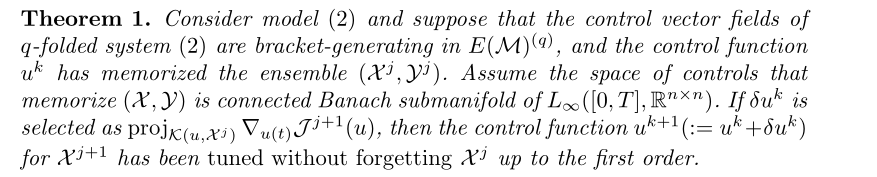
Tuning without Forgetting

Objective: Let $\mathcal{X}^{j}=\{x^{i}\in\mathcal{X}|i=1,2,\cdots,j\}$, and $\mathcal{Y}^j$ the corresponding batch of labels. Denote $u^k$ the control function at the $k$th iteration. Assume that $u^k$ has memorized the ensemble $(\mathcal{X}^{j},\mathcal{Y}^{j})$. We propose an iterative method to find a control $u^\ast$ such that

$$ C\varphi(u^*,x^i)=y^i \quad \text{for all} \quad x^i\in\mathcal{X}^{j+1}(=\mathcal{X}^j\cup\{x^{j+1}\}) $$

Tuning without Forgetting: Assume that $u^k$ has memorized the ensemble $(\mathcal{X}^{j},\mathcal{Y}^{j})$. If the update $\delta u^k$ satisfies

$$ \mathcal{J}^{j+1}(u^k+\delta u^k)\leq\mathcal{J}^{j+1}(u^k) $$

$$ R\left(\varphi(u^k+\delta u^k,x^i)\right)=y^i+o(\delta u^k),\quad \forall x^i\in\mathcal{X}^j $$

Then the control function $u^{k+1} := u^k + \delta u^k$ has been tuned for $\mathcal{X}^{j+1}$ without forgetting $\mathcal{X}^j$.

条件1：要求更新控制后，对新数据点的 cost 下降
条件2：要求更新控制后，对老数据点的影响不明显

A Projected Gradient Descent Method

Linearized Controllability Property: We say the system $\dot{x}(t)=f(x(t),u(t))$ has the Linearized Controllability Property (LPC) at $x^i$ for all $u\in L_{\infty}([0,T],\mathbb{R}^{n\times n})$ if the linear time varying system

$$ \dot{z}(t)=\left(\frac{\partial f(x,u)}{\partial x}\bigg|_{(x=\varphi_t(u,x^i),u)}\right)z(t)+\left(\frac{\partial f(x,u)}{\partial u}\bigg|_{(x=\varphi_t(u,x^i),u)}\right)v(t), $$

where $v(t)\in L_\infty([0,T],\mathbb{R}^{n\times n})$ is controllable.

LPC 是算法能正常运作的前提，其保证了非线性系统 $\dot{x} = f(x,u)$ 在局部线性化后，扰动可以被任意控制。

Impact of Updated Control: Suppose that a given control function $u$ has memorized the pair of points $(x^i, y^i)$, then

$$ \delta\varphi_t(u,x^i)=\int_0^t\Phi_{(u,x^i)}(t,\tau)\frac{\partial f(x,u)}{\partial u}\bigg|_{(x=\varphi_\tau(u,x^i),u)}\delta u(\tau)d\tau $$

up to first order in $\delta u(t)$. Here $\Phi_{(u,x^i)}(t, \tau)$ is the state transfer matrix defined by

$$ \frac{\mathrm{d}}{\mathrm{d}t}\Phi(t,\tau)=A(t)\Phi(t,\tau), \quad \Phi(\tau,\tau)=I $$

$$ A(t) = \frac{\partial f(x,u)}{\partial x}\bigg|_{(x=\varphi_t(u,x^i),u)} $$

上面的公式给出了如果我在各个 $\tau$ 时刻更新了控制为 $\delta u(\tau)$，那么最终的输出会变多少。

L Operator: Let $R$ be the readout function,

$$ \mathcal{L}_{(u,x^i)}(\delta u):=R\left(\int_0^T\Phi_{(u,x^i)}(T,\tau)\frac{\partial f(x(\tau),u(\tau))}{\partial u}\delta u(\tau)d\tau\right) $$

$\mathcal{L}$ 算子代表了 $\delta u$ 对最终输出的影响，如果希望不遗忘，则尽可能要让 $\mathcal{L}$ 算子为 $0$。

Null Space of L Operator:

$$ \mathcal{K}(u,x^i):=\operatorname{span}\{\delta u\in L_\infty([0,T],\mathbb{R}^{n\times n})\mid\mathcal{L}_{(u,x^i)}(\delta u)=0\} $$

$$ \mathcal{K}(u,\mathcal{X}^j):=\mathrm{span}\{\delta u\in L_\infty([0,T],\mathbb{R}^{n\times n})\mid\delta u\in\bigcap_{x^i\in\mathcal{X}^j}\mathcal{K}(u,x^i)\} $$

$\mathcal{K}$ 的价值在于只要我们选出了一个安全的子空间用于更新/投影

Projection Operator:

$$ \operatorname{proj}_{\mathcal{K}(u,\mathcal{X}^j)}\nabla_{u(t)}\mathcal{J}^{j+1}(u):=\arg\min_{d(t)\in\mathcal{K}(u,\mathcal{X}^j)}\int_{0}^{T}\|d(\tau)-\nabla_{u(\tau)}\mathcal{J}^{j+1}(u)\|^2d\tau $$

将理想学习方向 $\nabla_{u(t)}\mathcal{J}^{j+1}$ 投影到 $\mathcal{K}(u,\mathcal{X}^j)$ 中，从而构成更新方向，即 $\delta u=\mathrm{proj}_{\mathcal{K}}(\nabla_uJ^{j+1})$。这里的投影操作就是找了 $\mathcal{K}(u,\mathcal{X}^j)$ 中离 $\nabla_{u(t)}\mathcal{J}^{j+1}$ 距离最近的。

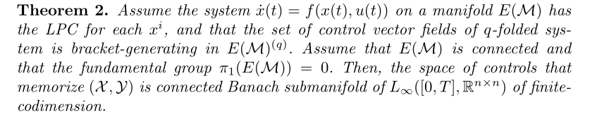
Main Results

Condition for Tuning without Forgetting:

More Detailed Condition:

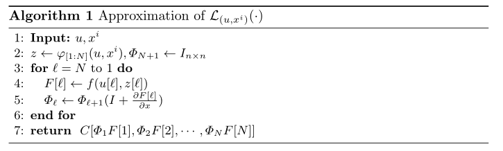
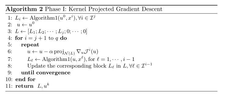
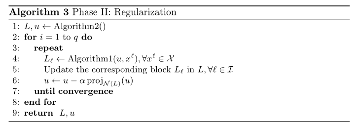
Numerical Methods

Approximation of $\mathcal{L}_{(u,x^i)}(\cdot)$: We provide a method to compute a numerical approximation of $\mathcal{L}_{(u,x^i)}(\cdot)$ for all $x^i \in \mathcal{X}^j$,

Phase 1 (Implement Theorem 1) :

Phase 2 (Minimize the Norm of **$u$** ) : In this phase, we project the gradient of the $L^2$ norm of the control function onto the subspace of functions $\mathcal{K}(u^k, \mathcal{X})$ at each iteration.

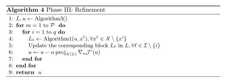
Phase 3 (Refinement) : In this phase, we aim to refine the control $u$ to steer all the points closer to their associated end-points. Let $\mathcal{P}$ be the number of iterations per sample.

‍