论文阅读:PINNs for PTV
Introduction
Particle Image Velocimetry: An optical measurement technique that determines an instantaneous velocity field by statistically analyzing the displacement of dense concentrations of tracer particles within interrogation regions over a short time interval.
PIV 追踪一块区域(interrogation window)的整体移动
Particle Tracking Velocimetry: An optical measurement technique that determines the pathways and velocities of individual tracer particles by identifying and tracking each particle over a sequence of images.
PTV 追踪单个粒子的精确轨迹
Limitation of PIV: PIV is generally limited by the size of the interrogation window and the number density of the recorded particles.
Limitation of PTV: The sparsity of the seeding particles also limits the spatial resolution achievable by PTV.
PINNs
Velocities: Assuming the velocities obtained from PIV/PTV are denoted as
$$ \mathcal{D}:\{\mathbf{x}^n,t^n,\mathbf{u}^n\}_{n=1}^{N_v}, $$
where $\mathbf{x}$ and $t$ are the space and time coordinates, $\mathbf{u}$ is the velocity, $N_v$ denotes the total number of vectors in the spatiotemporal domain $\Omega \times T$.
PINNs: A neural network $\mathcal{NN}$ is used to approximate the solution of the flow field
$$ (\mathbf{u},p)=\mathcal{NN}(\mathbf{x},t,\Theta). $$
where $\mathcal{NN}$ receives the coordinates as input and $\Theta$ is the learnable parameters in the network. $\mathbf{u}(\mathbf{x}, t, \Theta)$ and $p(\mathbf{x}, t, \Theta)$ are the velocity and pressure fields. In general, $\mathcal{NN}$ is instantiated by using a feed-forward fully connected network.
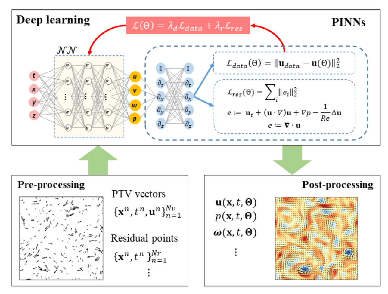
Data Loss: We apply the velocity data $\mathcal{D}$ as labels and minimize the mean squared loss:
$$ \mathcal{L}_{\mathrm{data}}(\Theta)=\sum_{(u,v,w)}\sum_{n=1}^{N}\parallel\mathbf{u}_{\mathrm{data}}^{n}-\mathbf{u}(\mathbf{x}^{n},t^{n},\Theta)\parallel_{2}^{2}. $$
This penalizes the mismatch between the data $\mathbf{u}_{\text{data}}^n$ and the network output $\mathbf{u}(\mathbf{x}^n, t^n, \Theta)$, where $\sum_{(u,v,w)}$ dentoes the summation over three velocity components, $\sum_{n=1}^{N}$ is the summation over different data points, and $N$ is the batch size for one training iteration.
Residual Loss: Another loss function penalizing the residuals of the governing equations is introduced:
$$ \mathcal{L}_{\mathrm{res}}(\Theta)=\sum_{i}\sum_{n=1}^{N}\parallel\mathbf{e}_{i}(\mathbf{x}^{n},t^{n},\Theta)\parallel_{2}^{2} $$
where $\mathbf{e}$ includes the residuals of the governing equations for flow motion. For instance, $\mathbf{e}_i$ can be
$$ \begin{aligned} & e_{1}=u_t+(uu_x+vu_y+wu_z)+p_x-1/\mathrm{Re}(u_{xx}+u_{yy}+u_{zz}) \\ & e_{2}=v_t+(uv_x+vv_y+wv_z)+p_y-1/\mathrm{Re}(v_{xx}+v_{yy}+v_{zz}) \\ & e_{3}=w_t+(uw_x+vw_y+ww_z)+p_z-1/\mathrm{Re}(w_{xx}+w_{yy}+w_{zz}) \\ & e_{4}=u_x+v_y+w_z \end{aligned} $$
Boundary Condition: If the boundary conditions of the investigated flow are known, we have
$$ \mathcal{L}_{\mathrm{bcs}}(\Theta)=\sum_{(u,v,w)}\sum_{n=1}^{N}\|\mathbf{u}_{\mathrm{bcs}}^{n}-\mathbf{u}(\mathbf{x}^{n},t^{n},\Theta)\|_{2}^{2}, $$
where $\{\mathbf{x}^n,t^n,\mathbf{u}_{\mathrm{bcs}}^n\}_{n=1}^{N_b}$ denote the Dirichlet boundary conditions on $\mathbf{x} \in \partial \Omega$.
Overall Loss Function: The loss function of PINN can be defined as
$$ \mathcal{L}(\Theta)=\lambda_d\mathcal{L}_{\mathrm{data}}+\lambda_r\mathcal{L}_{\mathrm{res}}+\lambda_b\mathcal{L}_{\mathrm{bcs}} $$
where $\lambda_\ast$ are the weighting coefficients used to balance different terms in the loss function.
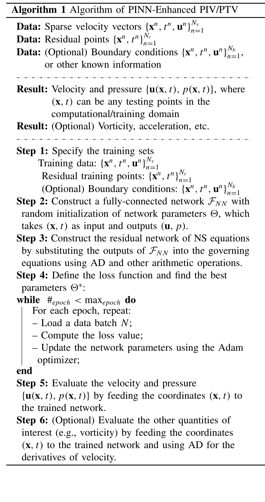
Generic Workflow in Real Experiments
Preprocessing: This step is to prepare the training sets in a proper format as required for PINN training. The velocity vectors loaded from PIV/PTV experiments are generally dimensionalized, so a nondimensionalization step is required:
$$ \mathbf{x}^*=\frac{\mathbf{x}}{L},\quad\mathbf{u}^*=\frac{\mathbf{u}}{U},\quad t^*=\frac{t}{L/U},\quad p^*=\frac{p}{\rho U^2}, $$
where $L$ is the length scale and $U$ is the velocity scale. Then $\{\mathbf{x}^{*n},t^{*n},\mathbf{u}^{*n}\}_{n=1}^{N_v}$ will be used in the data loss. Given the kinematic viscosity of the fluid $\nu$, the Reynolds number is defined as
$$ \mathrm{Re}=\frac{\mathrm{UL}}{\nu}. $$
If the boundary conditions are known, we can extract the boundary points $\{\mathbf{x}^{*n},t^{*n}\}_{n=1}^{N_{b}}$ and the corresponding velocity $\{\mathbf{u}_{\mathrm{bcs}}^{*n}\}_{n=1}^{N_{b}}$. Eventually, the training data are composed of
$$ \{\mathbf{x}^{*n},t^{*n},\mathbf{u}^{*n}\}_{n=1}^{N_{v}}, \quad \{\mathbf{x}^{*n},t^{*n}\}_{n=1}^{N_{r}}, \quad \{\mathbf{x}^{*n},t^{*n},\mathbf{u}_{\mathrm{bcs}}^{*n}\}_{n=1}^{N_{b}}. $$
Postprecessing: We generate an Euler mesh by defining the dimensionless time interval $\mathrm{d}t$ and spacing step $\mathrm{d} \mathbf{x}$. The evaluation points are defined as $(\mathbf{x}_{\mathrm{grid}}^*,t_{\mathrm{grid}}^*)$. Note that the flow fields should be dimensionalized back to the original units:
$$ \begin{aligned} (\mathbf{u}^{*},p^{*}) & =\mathcal{NN}\left(\mathbf{x}_{\mathrm{grid}}^{*},t_{\mathrm{grid}}^{*}\right) \\ \mathbf{u} & =\mathbf{u}^{*}\times U \\ p & =p^{*}\times\rho U^{2} \end{aligned} $$
where $(\mathbf{u}^{*},p^{*})$ are the dimensionless output of the last layer in the neural network and $(\mathbf{u},p)$ are the dimensional quantities which are used for visualization.