论文阅读:连续学习的最优控制方式
Original Paper: Optimal Protocols for Continual Learning via Statistical Physics and Control Theory
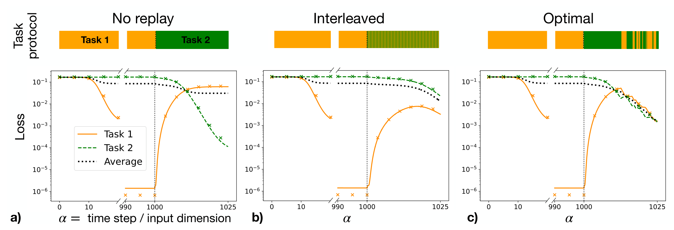
概述:本篇文章介绍了如何使用最优控制理论调整连续学习中的 Replay 任务、学习率使得最终的 generalization error 最低。
Introduction
Multi-Task Learning: Training a neural network on a series of tasks.
Catastrophic Forgetting: Multi-task learning can lead to catastrophic forgetting, where learning new tasks degrades performance on older ones.
Replay: Present the network with examples from the old tasks while training on the new one to minimize forgetting.
A Teacher-Student Framework
Teacher-Student Framework: Here we consider a teacher-student framework
Student: The student network is trained on synthetic inputs $\boldsymbol{x} \in \mathbb{R}^N$, drawn i.i.d. from a standard Gaussian distribution $x_i \sim \mathcal{N}(0, 1)$. It is a two-layer neural network with $K$ hidden units, first-layer weight $\boldsymbol{W} = (\boldsymbol{w}_1,\cdots,\boldsymbol{w}_K)^{\top} \in \mathbb{R}^{K \times N}$, activation function $g$, and second-layer weights $\boldsymbol{v} \in \mathbb{R}^K$. It outputs the prediction
$$ \hat{y}(\boldsymbol{x}; \boldsymbol{W}, \boldsymbol{v}) = \sum\limits_{k = 1}^K g \left( \frac{\boldsymbol{x} \cdot \boldsymbol{w}_k}{\sqrt{N}} \right). $$
Teacher: The labels for each task $t = 1,2,\cdots, T$ are generated by the teacher networks, $y^{(t)} = g_{\ast}(\boldsymbol{x} \cdot \boldsymbol{w}_{\ast}^{(t)}/\sqrt{N})$, where $\boldsymbol{W}_{\ast} = (\boldsymbol{w}_{\ast}^{(1)},\cdots,\boldsymbol{w}_{\ast}^{(T)})^{\top} \in \mathbb{R}^{T \times N}$ denote the corresponding teacher vectors, and $g_{\ast}$ the activation function.
Task-Dependent Weights: We allow for task-dependent readout weights $\boldsymbol{V} = (\boldsymbol{v}^{(1)},\cdots,\boldsymbol{v}^{(T)})^{\top} \in \mathbb{R}^{T \times K}$. Specifically, when the task $t$ is presented, the readout is switched to the corresponding task, the first-layer weights are shared across tasks.

Generalization Error: The generalization error of the student on task $t$ is given by
$$ \varepsilon_t(\boldsymbol{W}, \boldsymbol{V}, \boldsymbol{W}_*) := \frac{1}{2} \left\langle \left( y^{(t)} - \hat{y}^{(t)} \right)^2 \right\rangle = \frac{1}{2} \mathbb{E}_{\boldsymbol{x}} \left[ \left( g_* \left( \frac{\boldsymbol{w}_*^{(t)} \cdot \boldsymbol{x}}{\sqrt{N}} \right) - \hat{y}(\boldsymbol{x}; \boldsymbol{W}, \boldsymbol{v}^{(t)}) \right)^2 \right]. $$
where $(\boldsymbol{x}, y^{(t)})$ is a sample, $\hat{y}^{(t)}$ is the prediction, the angular brackets $\langle \cdot \rangle$ denote the expectation over the input distribution.
Overlaps Variables: The above generalization error depends only through the preactivations
$$ \lambda_k := \frac{\boldsymbol{x} \cdot \boldsymbol{w}_k}{\sqrt{N}}, \quad k = 1, \ldots, K, \qquad \text{and} \qquad \lambda_*^{(t)} := \frac{\boldsymbol{x} \cdot \boldsymbol{w}_*^{(t)}}{\sqrt{N}}, \quad t = 1, \ldots, T. $$
They define jointly Gaussian variables with zero mean and second moments given by
$$ \begin{aligned} &M_{kt} := \mathbb{E}_{\boldsymbol{x}} \left[ \lambda_k \lambda_*^{(t)} \right] = \frac{\boldsymbol{w}_k \cdot \boldsymbol{w}_*^{(t)}}{N} , \\ &Q_{kh} := \mathbb{E}_{\boldsymbol{x}} \left[ \lambda_k \lambda_h \right] = \frac{\boldsymbol{w}_k \cdot \boldsymbol{w}_h}{N} , \\ &S_{tt’} := \mathbb{E}_{\boldsymbol{x}} \left[ \lambda_*^{(t)} \lambda_*^{(t’)} \right] = \frac{\boldsymbol{w}_*^{(t)} \cdot \boldsymbol{w}_*^{(t’)}}{N} , \end{aligned} $$
called overlaps in the statistical physics literature. Therefore, the dynamics of the generalization error is entirely captured by the evolution of the readouts $\boldsymbol{V}$ and the overlaps.
Forward Training Dynamics: We use the shorthand notation $\mathbb{Q} = (\operatorname{vec}(\boldsymbol{Q}), \operatorname{vec}(\boldsymbol{M}), \operatorname{vec}(\boldsymbol{V})) \in \mathbb{R}^{K^2 + 2KT}$. The training dynamics is described by a set of ODEs
$$ \frac{\mathrm{d}\mathbb{Q}(\alpha)}{\mathrm{d}\alpha} = f_{\mathbb{Q}}(\mathbb{Q}(\alpha), \boldsymbol{u}(\alpha)), \quad \alpha \in (0, \alpha_F]. $$
The parameter $\alpha$ denotes the effective training time, and $\boldsymbol{u}$ is the control variable.
The Optimal Control Framework
Optimal Control Framework: Our goal is to derive training strategies that are optimal with respect to the generalization performance at the end of the training and on all tasks. In practice, we minimize a linear combination of the generalization errors on different tasks
$$ h(\mathbb{Q}(\alpha_F)) := \sum\limits_{t = 1}^T c_t \epsilon_t(\mathbb{Q}(\alpha_F)), \quad \text{with} \quad c_t \geq 0, \sum\limits_{t = 1}^T c_t = 1. $$
where $\alpha_F$ is the final training time, the coefficients $c_t$ identify the relative importance of different tasks and $\epsilon_t$ denotes the infinite-dimensional limit of the average generalization error on task $t$. We define the cost functional
$$ \mathcal{F}[\mathbb{Q}, \hat{\mathbb{Q}}, \bm{u}] = h\left(\mathbb{Q}(\alpha_F)\right) + \int_0^{\alpha_F} \mathrm{d}\alpha , \hat{\mathbb{Q}}(\alpha)^\top \left[ -\frac{\mathrm{d}\mathbb{Q}(\alpha)}{\mathrm{d}\alpha} + f_{\mathbb{Q}}\left(\mathbb{Q}(\alpha), \bm{u}(\alpha)\right) \right], $$
Here $\hat{\mathbb{Q}} = (\operatorname{vec}(\hat{\boldsymbol{Q}}), \operatorname{vec}(\hat{\boldsymbol{M}}), \hat{\operatorname{vec}(\boldsymbol{V}}))$ is the conjugate order parameters (We can consider it as a Lagrange multiplier that incorperates the dynamics of $\mathbb{Q}$).
Backward Conjugate Dynamics: